Global Optimization Portal - Algorithm | ||
The surrogate model software program developed at GOP is based on the methodolgy, mathematical formulation and software presented in RDIC.
In addition, a standard gradient-descent optimization routine is developed to carry out the search of global optimum location. The overview of the entire surrogate model based optimization process is given in the chart below.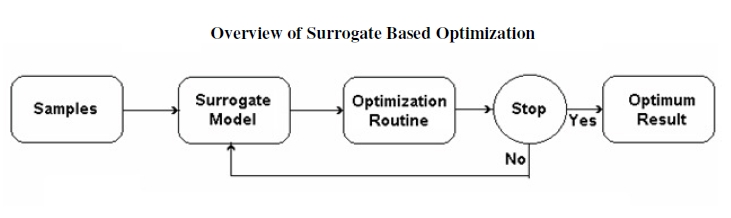 The structure chart of surrogate optimization process in terms of its components is presented in the following. 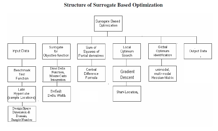 Dirac delta function is employed as a weighting function in the surrogate model. The Lorentz distribution function is chosen to approximate Dirac delta function in the computation process. easy to use. For example, in two dimensions at sample location (x', y'), the Dirac delta function can be written as,  Plotting the contour chart of the above formula by setting delta width Δ to 1 and rescaling by (π)2, it gives, 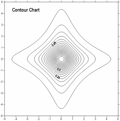 The center origin is located at the sample location (x', y') in the above chart. The abscissa is x-x' and the ordinate is y-y'. It is interesting to see that the contour lines near the origin form circular patterns (like L2 norm, the Euclidean norm) and beyond the origin change into shapes similar to diamond (like L1 norm, the Manhattan/taxicab norm). In contrast, IDW (Inverse Distance weighting) employs the L2 norm without pattern changes. Dirac delta function is symmetric. That is, δΔ(x'-x) = δΔ(x-x'). The surrogate model for the entire design space is constructed by using the target function values collected at the sample locations together with the weighting Dirac delta function, similar to the construction usd in IDW (inverse distance weighting) interpolation algorithm. However, unlike IDW which is ad-hoc, the mathematical construction of GOP surrogate model is based upon Monte Carlo method and the Central Limit Theorem. For details, check RDIC and the references listed there. For illustration, the surrogate model in one dimension can be written as follows. 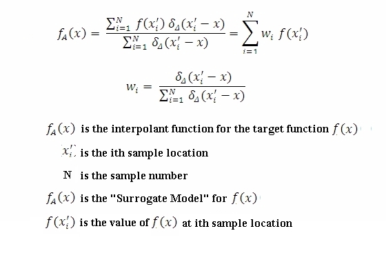 The accuracy of the interpolant is summarized here. (For details, see File C) The interpolant in the surrogate model can produce the target function values at any locations in the hypercube domain. All interpolated values will lie in between the maximum and the minimum of the input sample function values. This is due to the positive kernel property of the Lorentz distribution used in the interpolation process. The confinement of the interpolated values preclude the possibility to find the global maximum and minimum in the hypercube. However, the preclusion only holds when the delta width approaching zero (which also causes overfitting). By employing a finite delta width value as a smoothing parameter, it inevitably causes the shifting of the input extremum locations. The new extremum locations are formed due to the balance of competing forces from nearby (or far) sample points that produces the net, collective pull. The new location(s) are truly statistical outcomes but they possibly are moved towards the true optimum location. Of course, by changing the delta width the new location will change again. Thus, it is critical to treat the new locations with caution. The better way to handle the matter is to run with 2 or 3 different delta width values (not much bigger than the default value in order to avoid underfitting). Compile the new locations and evaluate these candidate locations by using the actual analytic function, simulation program or experiments for the ground truth check. After completing this workflow, one can select the best optimum answer for the given input data. In fact, the three examples presented in GOP-Resource verified the applicability of the proposed strategy of optimum finding. The following table captures the global optimum (minimum) findings of the three examples in 1-D, 2-D and 4-D hypercubes. The true target function values at these global minimum locations are given and compared with the input sample function values at their minimum locations. The newly found extremum (optimum) locations are better than the extremum locations in the input samples, even though the interpolated values via the surrogate model at the the new extremum have higher function values than the input sample function minima. The results validated the GOP optimization algorithm and procedure, as well as its merit.  GOP interpolant not only computes the interpolated function values but also provides the confidence intervals (one sigma, three sigma) same as in Kriging method. The formulas to compute confidence intervals are briefly summarized below. For details including all the equations used, read the file in RDIC. 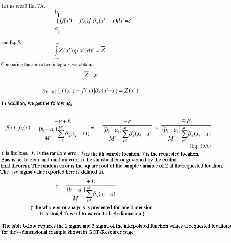 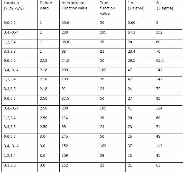 COMMENTS: It can be seen that at location (0,0,0,0) with delta=1 (which is smaller than the default 2.18 value) gives a very small sigma value. This happens because it coincides with one of the input sample location. If delta value is approaching zero, so does the sigma value at this location. At other locations, the sigma values are moderate at different delta values. With more input samples, the sigma value will come down in accordance with the central limit theorem. Generally speaking, the delta value should be set near the default value. GOP employes the gradient descent method to find the optimum. Even with moderate sigma values, the gradient values are acceptable because they measure the local change rates (the slopes) of the target function. Interpolated function values of two nearby locations will likely have more or less the same sigma offset and it will not impact much the derivative calculation. |
© FANG, INC. 2026 All Rights Reserved
(All information including software provided at GOP should be used by the discretion of the user.
FANG, INC. is not responsible for the outcome of the usage of GOP.)