 Eq. (A)
            (x-x2)(x-x3)(x-x4)f(x1)              (x-x3)(x-x4)(x-x1)f(x2)
 fA(x) =   ----------------------------    +  ---------------------------
            (x1-x2)(x1-x3)(x1-x4)                 (x2-x3)(x2-x4)(x2-x1)

               (x-x4)(x-x1)(x-x2)f(x3)           (x-x1)(x-x2)(x-x3)f(x4)
           + ----------------------------  +  ----------------------------
              (x3-x4)x3-x1)(x3-x2)	        (x4-x1)(x4-x2)(x4-x3)

where  a < x < b ;
In the above formula, f(x1), f(x2), f(x3), f(x4) and x1, x2, x3, x4 are given. Generalization of the formula to higher number of points is straightforward. It can be seen that by specifying x value in the interval, the formula produces fA(x) value. The function f(x) is approximately represented by the interpolant fA(x) for the interval (a, b). Note that every f(xi) has a contribution to fA(x) value. In essence, fA(x) is in the form of polynomial. It needs to be said that the interpolant above can not be deduced, and therefore it is not simple to be extended to 2-dimension and above.Our formulation begins with the observation that the following equation exists,
 Eq. (A)
where x is the arbitrary value of x' variable and a1< x <b1 and  is the well-known Dirac delta function which is peaked symmetrically at x'= x and has the analytic form, (This form is called "Lorentzian" in physics and "Cauchy density" in statistics.)

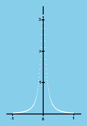
where  is the delta width which controls the width of the peak and is a small value, and f(x) is any continuous function in the interval. A sample picture of Dirac delta function is displayed below. Note that when x'-x = ±
 ,
,  has half its peak value. Furthermore, by substituting (Eq. B) into (Eq. A), the integral becomes,
 (Eq. A-1)
where  is a finite number. As
  goes to zero, so does
  .
.
The abscissa is x' axis and the ordinate is the approximated Dirac delta function of (Eq. B)
(In the picture,  =0.1 and x=0.0)

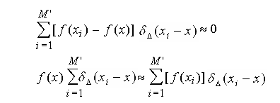
We now recast Eq. (A-1) by use of the standard Monte-Carlo method to replace the integral by an algebraic sum and suppressing the  term, it gives,
 Eq. (C)

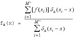
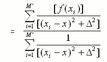
 Eq. (D)
fA(x) is the interpolant for the function f(x). Note that each f(xi) has a contribution to fA(x). M' is the value of random locations. As can be seen in Eq. (D), the only input data needed to numerically generate fA(x) are: M' value,  value, xi values, f(xi) values and x value. The derivation of our interpolant for 2-dimension space is straightforward, as well as for any higher dimension (Please read other sections). For two-dimension, our interpolant has the form,
 Eq. (E)
Check Sample Cases provided in RDIC to find out typical M' and  values for different dimensions. Note that our formulation only requires the use of random sampling (whether irregularly or regularly spaced), and it is independent of any particular sampling technique. Thus, our interpolant can be employed by any improved sampling methods such as stratified sampling, quasi Monte-Carlo sampling, etc. to produce better interpolants. Accuracy and convergence analysis of our interpolants are documented and downloadable. It should be pointed out that our interpolant does not involve any "coefficients" or "root finding" that need to be determined before the interpolation can take place, in contrast to conventional interpolation methods where product splines, polynomials, orthogonal expansions and RBF (radial basis function) method were used. In addition, the software which implements our interpolant has an unusual small size and that makes online, fast response calculation over the Internet a reality.
© FANG, INC. 2002-2004 All Rights Reserved